Difference between revisions of "Metabolic control analysis example"
(→Reproducing a test case in BioUML) |
|||
| (11 intermediate revisions by one user not shown) | |||
| Line 1: | Line 1: | ||
| + | <font size="3"> | ||
| + | |||
The method description could be found in the section [[Metabolic Control Analysis]]. Here we give an example of the method application and using in BioUML. | The method description could be found in the section [[Metabolic Control Analysis]]. Here we give an example of the method application and using in BioUML. | ||
==Reproducing a test case in BioUML== | ==Reproducing a test case in BioUML== | ||
| − | To reproduce a test case below in [[BioUML]] workbench | + | To reproduce a test case below in the [[BioUML]] workbench, go to the <b>Analyses</b> tab in the navigation pane and follow to ''analyses'' > ''Methods'' > ''Differential algebraic equations''. |
After double click on ''Metabolic Control Analysis'', a new tab with analysis settings opens. | After double click on ''Metabolic Control Analysis'', a new tab with analysis settings opens. | ||
| − | Select a path to | + | Select a path to the input diagram: |
''data/Examples/DAE models/Data/Diagrams/Geva_Zatorsky_2006_Model_I'' | ''data/Examples/DAE models/Data/Diagrams/Geva_Zatorsky_2006_Model_I'' | ||
| Line 13: | Line 15: | ||
and a path to save results of analysis, for example: | and a path to save results of analysis, for example: | ||
| − | ''data/Collaboration/Demo/Data/Temp/Metabolic Control Analysis'' | + | ''data/Collaboration/Demo/Data/Temp/Metabolic Control Analysis Results'' |
| − | After you click the ''Run'' button and the calculations are finished, you can see the results presented in six tables, including unscaled elastisities (the matrix ''Ɗ<sub>C<sup>ss</sup></sub>v'' in the description below), unscaled concentration controls (the matrix Γ), unscaled flux controls (the matrix Λ), and scaled versions of these matrices with elements ''e<sub>i,j</sub>'' defined as a product of the corresponding elements | + | <br>[[File:mca_figure_1.png]]<br><br> |
| + | |||
| + | After you click the ''Run'' button and the calculations are finished, you can see the results presented in six tables, including unscaled elastisities (the matrix ''Ɗ<sub>C<sup>ss</sup></sub>v'' in the description below), unscaled concentration controls (the matrix Γ), unscaled flux controls (the matrix Λ), and scaled versions of these matrices with elements ''e<sub>i,j</sub>'' defined as a product of the corresponding elements in the unscaled matrixes and values of ''c<sub>i,j</sub> / r<sub>i,j</sub>'', where ''c<sub>i,j</sub>'' and ''r<sub>i,j</sub>'' denote steady state values of column and row elements, respectively. | ||
Ready analysis results can be found here: | Ready analysis results can be found here: | ||
| − | data/Examples/DAE models/Data/Metabolic Control Analysis | + | ''data/Examples/DAE models/Data/Metabolic Control Analysis Results'' |
==Description of the test case== | ==Description of the test case== | ||
| Line 72: | Line 76: | ||
==References== | ==References== | ||
# Reder C. Metabolic control theory: a structural approach. ''Journal of Theoretical Biology''. 1988. V. 135. № 2. p. 175-201. | # Reder C. Metabolic control theory: a structural approach. ''Journal of Theoretical Biology''. 1988. V. 135. № 2. p. 175-201. | ||
| + | |||
| + | </font> | ||
Latest revision as of 10:48, 16 March 2022
The method description could be found in the section Metabolic Control Analysis. Here we give an example of the method application and using in BioUML.
[edit] Reproducing a test case in BioUML
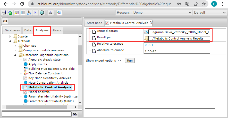
To reproduce a test case below in the BioUML workbench, go to the Analyses tab in the navigation pane and follow to analyses > Methods > Differential algebraic equations.
After double click on Metabolic Control Analysis, a new tab with analysis settings opens.
Select a path to the input diagram:
data/Examples/DAE models/Data/Diagrams/Geva_Zatorsky_2006_Model_I
and a path to save results of analysis, for example:
data/Collaboration/Demo/Data/Temp/Metabolic Control Analysis Results
After you click the Run button and the calculations are finished, you can see the results presented in six tables, including unscaled elastisities (the matrix ƊCssv in the description below), unscaled concentration controls (the matrix Γ), unscaled flux controls (the matrix Λ), and scaled versions of these matrices with elements ei,j defined as a product of the corresponding elements in the unscaled matrixes and values of ci,j / ri,j, where ci,j and ri,j denote steady state values of column and row elements, respectively.
Ready analysis results can be found here:
data/Examples/DAE models/Data/Metabolic Control Analysis Results
[edit] Description of the test case
The theory of metabolic control determines sensitivity of steady metabolic fluxes (reaction rates) vss and steady state Css of an ODE model under perturbation of its parameters K [1]. Unlike the Sensitivity Analysis, this method does not require the computation of values Css(p + Δp), p ∈ K, that can accelerate the model research. Instead, to analyze matrixes ƊKCss and ƊKvss of partial derivatives of Css and vss with respect to parameters K, the method considers a matrix ƊKv|C(t) = Css of partial derivatives of a vector v(t) with respect to K in a steady state of the model, and searches for control matrices Γ and Λ, such that
In accordance with [1], these matrices can be calculated by formulas
where NR is a matrix consisting of linearly independent rows of the model stoichiometric matrix N of n by m, L is a transition matrix such that: N = L · NR, and ƊCssv is a matrix of elasticity coefficients
Consider the model of p53 and Mdm2 proteins regulation described in the example for Sensitivity Analysis. For this model, we get:
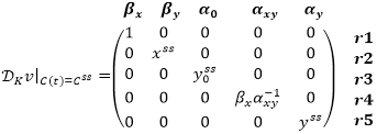
Next, we find the matrixes N and ƊCssv:
Since NR = N and L is the identity matrix of 3 by 3, we can calculate the matrix product N · ƊCssv:
Applying the cofactor method to the resulting matrix, we deduce:
Thus, we have:
Take into account the formulas for calculation of the model steady state derived in the Sensitivity Analysis example:
Using these formulas, we can convert matrix Γ to the form:
Multiplication of the calculated matrices Γ and ƊKv|C(t) = Css gives the same matrix ƊKCss, as in the example for Sensitivity Analysis:
[edit] References
- Reder C. Metabolic control theory: a structural approach. Journal of Theoretical Biology. 1988. V. 135. № 2. p. 175-201.


