Optimization problem

The general nonlinear optimization problem [1] can be formulated as follows: find a minimum of the objective function ϕ(x), where x lies in the intersection of the N-dimensional search space

and the admissible region ℱ ⊆ ℝ^N defined by a set of equality and/or inequality constraints on x. Since the equality g_s(x) = 0 can be replaced by two inequalities g_s(x) ≤ 0 and –g_s(x) ≤ 0, the admissible region can be defined without loss of generality as

In order to get solution situated inside ℱ, we minimize the penalty function

The problem could be solved by different optimization methods. We implemented the following of them in the BioUML software:

• stochastic ranking evolution strategy (SRES) [1];
• cellular genetic algorithm MOCell [2];
• particle swarm optimization (PSO) [3];
• deterministic method of global optimization glbSolve [4];
• adaptive simulated annealing (ASA) [5].

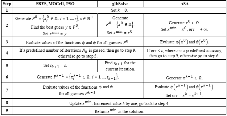
The below table shows the generic scheme of the optimization process for these methods. SRES, MOCell, PSO and glbSolve run a predefined number of iterations N_it considering a sequence of sets (populations) Pⁱ, i = 0,…,N_it − 1, of potential solutions (guesses). In the case of the first three methods, the size s ∈ ℕ⁺ of the population is fixed, whereas in glbSolve the initial population P⁰ consists of one guess, while the size s_{k+ 1} of the population P^k+1 is found during the iteration with the number k = 0,…, N_it − 1. The method ASA considers sequentially generated guesses x^k ∈ Ω, k ∈ ℕ⁺, and stops if distance between x^k and x^k+1 defined as Euclidean norm

becomes less than a predefined accuracy ε.

All methods, excepting glbSolve, are stochastic and seek global minimum of the function ϕ taking into account the admissible region ℱ. Thus, a guess x ∈ Ω is more preferable than a guess y ∈ Ω at some iteration of methods, if ψ(x) = 0 and ψ(y) ≠ 0 or ψ(x) < ψ(y). The method glbSolve is suited to solve only the problems with Ω ⊆ ℱ. Values of the function ψ are calculated but do not affect on the generation of potential solutions.

Application of non-linear optimization to systems biology

We assume that a mathematical model of some biological process consists of a set of chemical species S = {S₁,…,S_m} associated with variables C(t) = (C₁(t),…,C_m(t)) representing their concentrations, and a set of biochemical reactions ℛ = {R₁,…,R_n} with rates v(t) = (v₁(t),…,v_n(t)) depending on a set of kinetic constants K. Reaction rates are modeled by standard laws of chemical kinetics. A Cauchy problem for ordinary differential equations representing a linear combination of reaction rates is used to describe the model behavior over time:

   (*)

Here N is a stoichiometric matrix of n by m. We say that C^ss is a steady state of the system (*) if

Identification of parameters K and initial concentrations C⁰ is based on experimental data represented by a set of points C_i^exp(t_i,j) defining dynamics of variables C₁(t),…,C_l(t), l ≤ m, at given times t_i,j, j = 1,…,r_i, where r_i is the number of such points for the concentration C_i(t), i = 1,…,l. The problem of parameter identification consists in minimization of the function of deviations defined as the normalized sum of squares [6]:

where normalization factors ω_min/ω_i with ω_min = min_iω_i are used to make all concentration trajectories have similar importance. The weights ωi are calculated by one of the formulas on experimentally measured concentrations:

(mean square value), (mean value), (standard deviation).

If we want to consider additional constrains

holding for concentrations C(t) and parameters K for some period of time , the penalty function is defined as

References

1. Runarsson T.P., Yao X. Stochastic ranking for constrained evolutionary optimization. IEEE Transactions on Evolutionary Computation. 2000. 4(3):284–294.
2. Nebro A.J., Durillo J.J., Luna F., Dorronsoro B., Alba E. MOCell: A cellular genetic algorithm for multiobjective optimization. International Journal of Intelligent Systems. 2009. 24(7):726–746.
3. Sierra M.R., Coello C.A. Improving PSO-Based Multi-objective Optimization Using Crowding, Mutation and ∈-Dominance. Evolutionary Multi-Criterion Optimization. Lecture Notes in Computer Scienc. 2005. 3410:505-519.
4. Björkman M., Holmström K. Global Optimization Using the DIRECT Algorithm in Matlab. Advanced Modeling and Optimization. 1999. 1(2):17–37.
5. Ingber L. Adaptive simulated annealing (ASA): Lessons learned. Control and Cybernetics. 1996. 25(1):33–54.
6. Hoops S., Sahle S., Gauges R., Lee C., Pahle J., Simus N., Singhal M., Xu L., Mendes P., Kummer U. COPASI-a COmplex PAthway SImulator. Bioinformatics. 2006. 22(24):3067–3074.